Projects and experiments
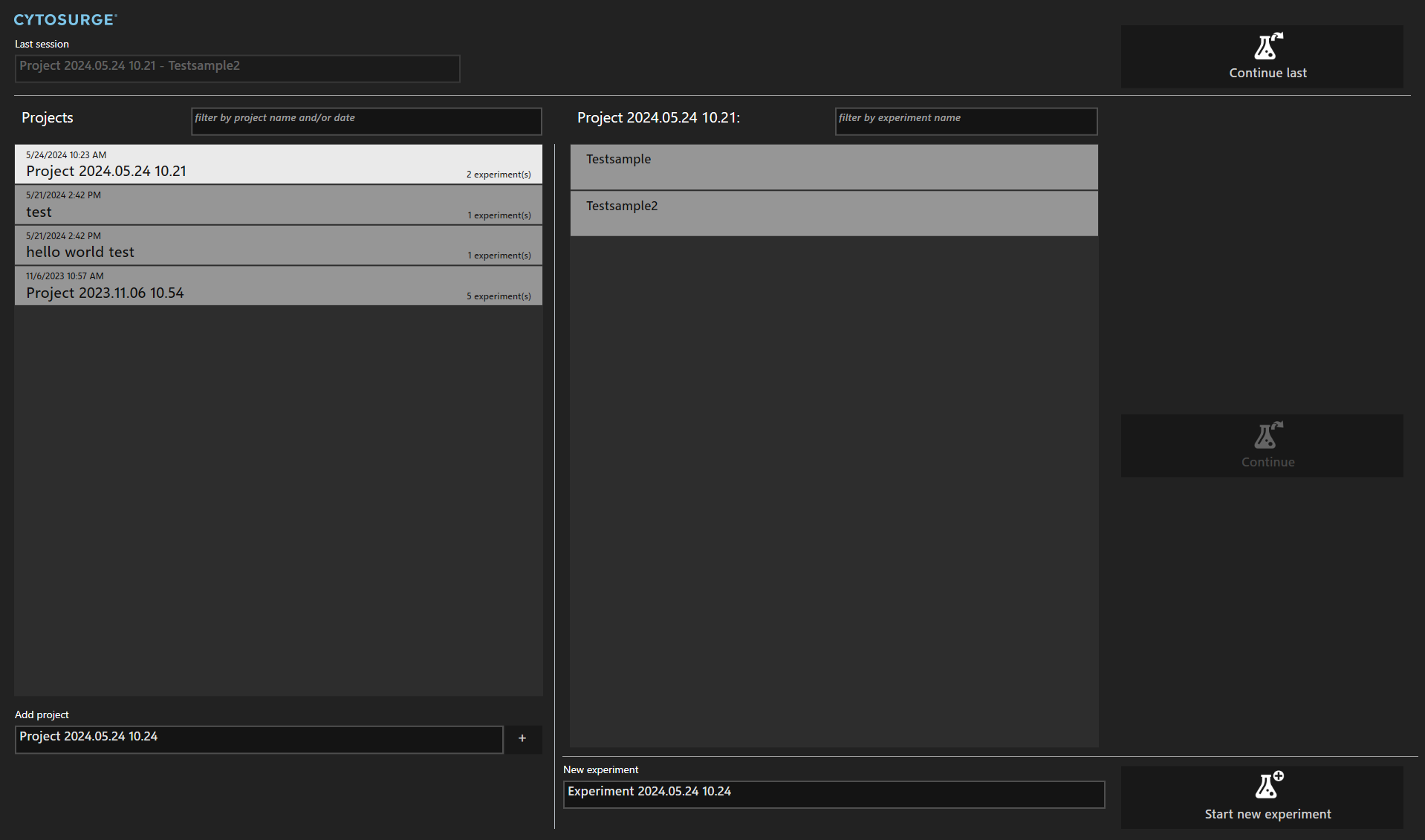
After starting the application, you are presented with the project dialog. You can create a new project, create a new experiment or continue an experiment. They are useful to group results.
Project
A project is a collection of experiments and helps you grouping similar experiments.
Experiment
An experiment groups the results of your research. There can be multiple experiments assigned to a project.
It is possible to resume experiments. However, certain environmental parameters may have changed and need to be taken into account when doing so: If plates are re-inserted, points recorded in a previous session might show a positioning offset when being accessed again or a different spring constant applies if another probe is mounted.
To avoid plate mixups the software supports assignment of plate identifiers on an experiment level. If set, the identifiers will be displayed in the experiment list.
Searching/Filtering
The list of projects and the list of experiments can be filtered by search words. This search is case insensitive. You may enter multiple words, then the names must contain all words in any order. Projects can also be filtered by their creation date. When the experiments are search it will only show the projects that have an experiment that contains these search words.
For example:
- the search word
testshows all projects, or experiments respectively, that contain the wordtest. test hellowill find the projecthello world test.test 2024finds all projects that contain the wordtestin its name and are created in 2024.11/6finds the projects created on the 6th of November.- When searching experiments for
sample, only the projects are shown that have an experiment that containssamplein its name and the experiments list is also filtered by this word.
Tools
Toolbar
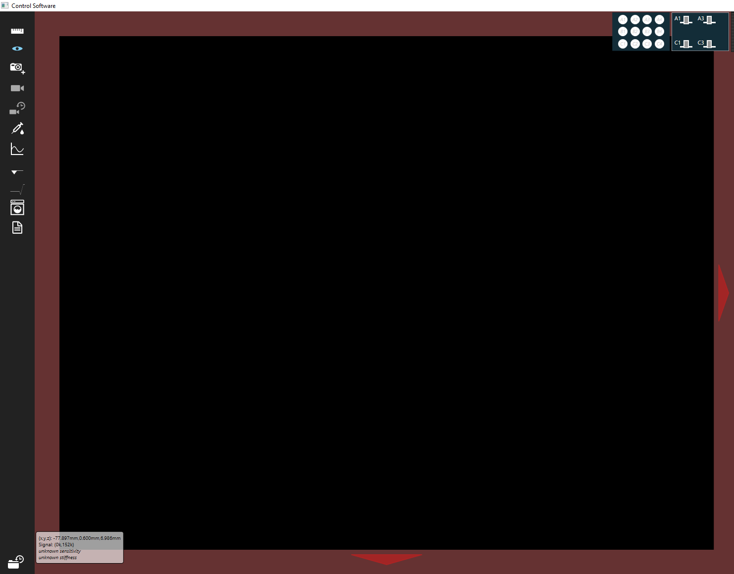
The toolbar is located on the left side of the main window and gives quick access to a set of functions described below:
| Tool | Name | Description |
|---|---|---|
 |
Scalebar | Toggles the scale bar at the bottom of the sample display |
 |
Navigation tool | Tool to navigate the worktable |
 |
Take screenshot | The screenshot of the current microscope image can be exported later in different formats |
 |
Take screenshot with specific settings | |
 |
Record a video | |
 |
Save Video History | Save last few seconds |
 |
Pressure tool | Manual pressure control |
 |
Oscilloscope | Shows signal streams |
 |
Probe tool | Manual z positioning |
| Spectroscopy tool | User-programmable z positioning | |
 |
Wash tool | Save and run wash cycles |
 |
Record a note | |
 |
Preset tool | Save and restore settings |
 |
Show Result Data | |
 |
Cell Volume Calculator | Perform volume calculations on injected cells |
 |
Cantilever Volume Calculator | Perform volume estimation on cantilever images |
 |
Video difference tool | Show image difference around cantilever area |
| Cell tracking tool | Track cells in a time series |
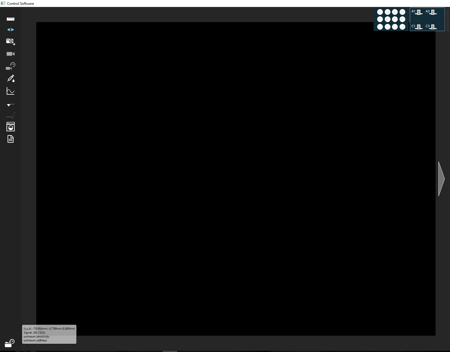
Navigation tool
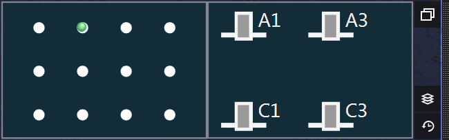
The navigation tool indicates the current position of the probe as a green circle in the active plate configuration.
Positioning
The tool can be used to move the probe into any of the wells by clicking inside the well with the mouse. The effecive target position of the probe depends on the size and contents of the clicked well:
Relative
In general, the probe moves to the position inside the well where the mouse click occurs.
Well center
When targeting a small well, the probe is automatically moved to the center of the well. Any well with a reachable area whose X- and Y-dimensions are less than 7mm is considered small. Please refer to the plate editor for distinction between reachable area and physical well size.
For any other well, the same can be achieved by holding down the Shift key while clicking inside the well.
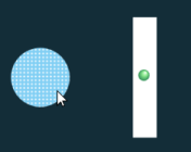
When the mouse is above a well, a cross in the well’s center indicates that the probe will move to the center:
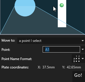
Point based
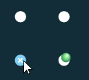
When the well contains a point pattern, the well is marked with white dots:
Clicking on such a well will give you a wider choice of possible targets:
- the well’s center
- the center of the point pattern’s
- any point in the point pattern
- a point relative to the well’s center
Note
To use custom plates, have a look a the plate editor to create a model for the control software.
Collision avoidance
For certain combinations of plates there is a risk of the Omnium head colliding with one of the plates when moving into a well. In this case, the affected wells are disabled and the area with a collision risk is grayed out in the plate view:

The software does not allow you to move to disabled wells.
Activity Map
The activity map can be toggled using the  button on the right.
It displays previously processed positions which have a result attached in the plate view.
Usually the positions are too close to each other to be displayed as single points in the overview.
Instead, a black rectangular area indicates the approximate position of possibly multiple processed positions in a well.
button on the right.
It displays previously processed positions which have a result attached in the plate view.
Usually the positions are too close to each other to be displayed as single points in the overview.
Instead, a black rectangular area indicates the approximate position of possibly multiple processed positions in a well.
Pressing any of the Ctrl keys on the keyboard zooms in on the area of the plate under the mouse:
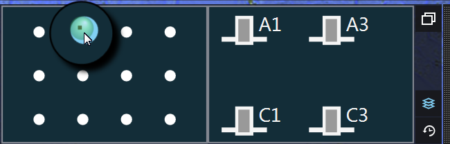
- Activity map shown in navigation tool with zoom enabled through the ‘Ctrl’-key
The points displayed in the activity map can be restricted using the point overlay control in the status bar.
Navigation History
A click on the bottom right button reveals the navigation history. It lists previously used positions.
Entries are added automatically when using the navigation tool to move to new positions. You can also manually add an entry
by clicking the  button below the list.
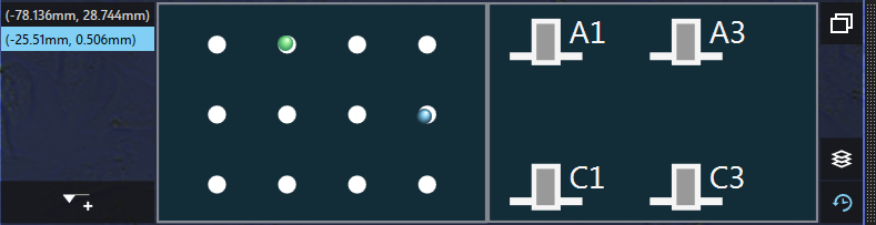
You can move to a previously used position by selecting it in the list and then clicking on the blue circle displayed on the plate.
Take screenshot with specific settings
After pressing this icon choose a preset from the list that pops up. The system will then temporarily apply the selected settings, save an image and revert the settings to their original state.
Make a video
Pressing this icon triggers the recording of the current microscope image. Accordingly, the record icon is displayed until you click again to cap the recording.
Note
Overlay information and currently shown controls like the cross-hair will not be included in the movie. Movies are not stored in the database because they are too big. Instead, they are directly exported to the corresponding folder.
Save past 30s
This tool allows you to conveniently save an unexpected event on video even after it occurred. By clicking the icon the past 30 seconds of your video feed are recovered and saved at a reduced frame rate.
Pressure tool
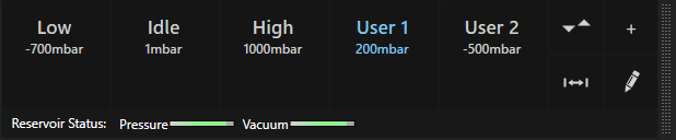
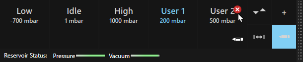
This tool allows you to directly control the pressure applied to the cantilever. The currently active pressure is highlighted in blue.
You can add, edit or delete custom pressure values by using the corresponding buttons on the right.
 Add
Add
Adds the current target pressure to the list of custom pressure values. You can directly change the pressure value using the number pad. Custom pressures are stored between sessions.
 Edit
Edit
Enters “edit mode”: move the mouse over a custom pressure and click the pen to edit its value or click the ‘X’ to delete it.
If you change an active pressure value, the new value is applied immediately.
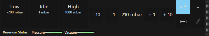
 Show up-down control
Switches to the up-down view where you can change the target pressure in small steps.
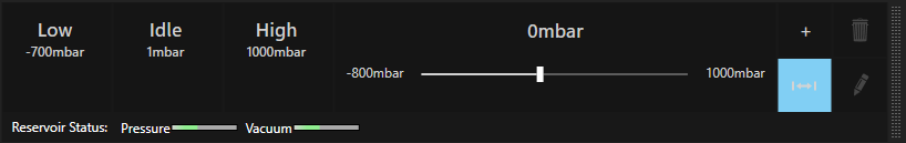
 Show slider
Switches to the slider view where you can change the target pressure using a slider.
Additionally, the status of the pressure reservoir is indicated at the bottom, where a full bar (green) signals that the operational pressure levels are reached in the reservoirs.
Oscilloscope
The oscilloscope icon toggles an animated graph which displays the deflection and the pressure of the last few seconds.
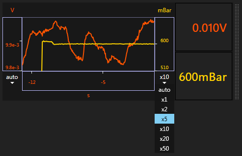
Right next to the graph, you can see the current values of the deflection and the pressure.
The scaling of the rulers on either side can be adjusted. Per default, it will automatically scale to show all recent values. If you would like to see a fixed total range, you can adjust the zoom by expanding the zoom combo box and choosing a value. Additionally, you can just use your mouse scroll wheel to scroll through all available zoom levels.
Note that the deflection signal always shows uncorrected values. Therefore, one will observe a corresponding shift of the signal when applying a relative setpoint but the signal itself will not necessarily correspond to that setpoint.
Probe tool
Probe-related positioning options (left to right):
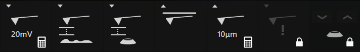
- Approach: Pressing triggers an approach operation to the configured setpoint; pressing the icon again aborts the operation
- Content Height: Pressing triggers a movement to the corresponding plate’s
content height. Pressing the icon again aborts the movement. - Focus on Probe: Attempts to bring the probe into focus. Button is only available if calibration data is available and the mircoscope is motorized.
- Home position: Retracts the FluidFM probe to the uppermost position. Pressing the icon again aborts the movement.
- Retract: Retracts the probe by the configured distance. Pressing the icon again aborts the movement.
- Advance: Moves the cantilever quickly towards the sample; a second click aborts the movement. Due to the high crash risk, the operation must first be unlocked by clicking on the lock.
- Focus: Tool to move the active lens outside of its configured focus limit.
 Spectroscopy tool
This tool allows you to quickly define and carry out a force spectroscopy.
It can be used to optimize the spectroscopy parameters used in the workflows or to run ad-hoc motion profiles.
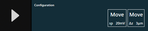
How to use:
- First, click on the surface next to the triangle/”play” symbol to load the configuration dialog
- Second, click on the triangle/”play” symbol to start executing your program
- Finally, you can have a look at the resulting curve displayed below the tool
A spectroscopy curve taken with the tool is not automatically saved; pressing the save icon next to the curve moves it to the result history.
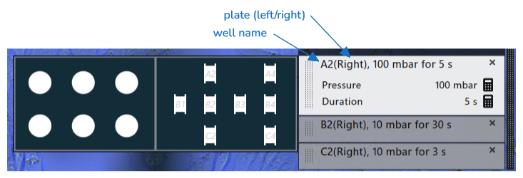
Wash tool
The wash tool allows you to set up a wash cycle using wells on the probe plate (except the probe holder locations) or any other plate.
The idea is to first fill empty, unused wells with washing solutions of your choice and then define a dipping time and a pressure value you wish to apply during the dipping step.
Unless Return to current position after washing is checked, the probe remains in the last container to avoid drying out.
As an example, you could have:
- Bleach in well A2, 5s at 100mbar
- Water in well B2, 30s at 10mbar
- Water in well C2, 2s at 0mbar (the probe will stay here).
You can define several such wash sequences with each having a name of your choice.
Note
Please make sure that the wells contain enough liquid: The probe will move down to about 2mm from the well bottom.
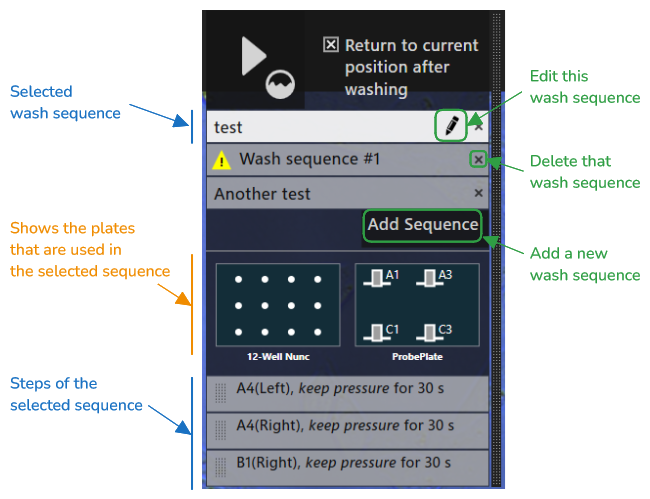
A warning ![]() is shown if the sequence is not applicable with the current plates.
is shown if the sequence is not applicable with the current plates.
Creating or editing a wash sequence
-
To add a new wash sequence click
Add Sequence. The order of the sequences is not relevant. You can change the order by dragging them to the desired position. -
To edit a wash sequence, select it and then click on
 .
.- Change the name of the sequence by editing the text field.
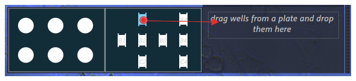
- To add a new wash step to the sequence: click on a well in the plate view and drag it to the sequence.
- To change the pressure or duration of a wash step: first select the step you want to modify, then click on the property you want to edit.
- By default, the pressure is set to keep, which means that the pressure that has last been applied remains unchanged when this step is started.
- To change the pressure back to keep, modify the pressure and delete all numbers.
- To change the position of a step in the sequence: click on the dotted area of a step and drag it to the new position.
Click on the “wash” button to start the wash cycle:

Return to current position after washing remembers the position of the probe before starting the wash cycle and
moves the probe back to this position once the wash cycle finishes.
Persistence
The wash sequences are saved when the control software is closed and are loaded again the next time you open the wash tool.
Record Note (Text tool)
You can take a short text note during your experiment by using the Text tool. It will be saved in the result history and be available later when you are reviewing the data. In that sense, you can use the Text tool as a built-in lab journal.
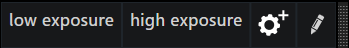
Preset tool
This tool allows you to store current settings to a preset and restore the saved settings at a later time. This empowers you to switch between different settings quickly without having to change all settings manually.
Click on the  button to save the current settings to a new preset. You will be presented with a window asking you for a name for the preset and showing the list of settings that will be stored. You must choose a different name for each saved preset. Saved presets will be available again after restarting the software.
Clicking on a preset will immediately apply the stored settings.
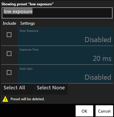
Click on the  button to enter “edit mode”: when in this mode, click on a preset to view the settings without applying them. In the opened dialog, the preset’s name can be changed and individual settings can be removed. If all settings are removed, the whole preset is deleted.
Result history
All your results (such as force curves and screenshots, except recorded videos) are stored in the database. You can view the stored results of the current experiment in the result history.
If you click on a preview icon or thumbnail an enlarged view with the full details of the result will open. This will also enable you to export the result to a file.
The result history offers different view modes, which can be chosen at the bottom of the result history:
 Single column
Displays the result previews in a compact single column next to the tool bar.
 Extended column
Displays the result previews in a single column as above, but with a few informative details:
- An Id of the result in the database
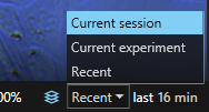
- The date and time (in minutes) when the result was acquired
- The time since the first result of the experiment was acquired
 Multiple columns
Presents result previews in multiple columns, such that more results are visible compared to single column mode.
Export... supports export of single and multiple items. Shift+click to select a range of items, Ctrl+click to select multiple, individual items.
Export all... exports all results from the current experiment.
 Point filter
Allows you to filter results by position. This view is only useful in conjunction with points that were saved during the review step of the Injection workflow or after saving points during position selection.
Select a point in the upper part to see a preview of all results associated with this point. This will also enable you to directly export all these results.
Note
If a point occurs in more than one point group, selecting it will highlight it in all groups
To select (or deselect) a group of points click on the group’s name to the left of the points. This will show all results associated with the points of the selected group and allows you to export all these results at the same time. You can select and export multiple groups in this way.
Video difference tool
This tool allows you to highlight changes in the video feed in a selected area by subtracting each video
frame from a reference image taken upon opening of the tool.
The  button can be used to set a new reference image
at any time.
button can be used to set a new reference image
at any time.
Two different modes are supported:
 Custom rectangle
After choosing this mode a rectangle can be drawn on the video view to define the area of the video for which the difference should be computed.
 Cantilever
In this mode the tool automatically selects an area around (and including) the cantilver. An outline of the cantilever’s inner bounds including graduation marks indicating the inner volume is overlaid on the image.
- Positioning
- This outline and the image area are positioned according to the probe’s opening as determined by align probe.
- Volume
- The volume inside the cantilever is the result of the active channel height multiplied by the fixed width plus the volume of the pyramid. The graduation marks are also adjusted according to the cantilever’s pitch (11°).
System Information
Located below the video feed, this tool displays system status information
- Currently applied pressure.
- Current axes position as a (x,y,z) tuple. Note that erroneous values might be reported while an initialization procedure takes place.
- Currently measured ADC values and the resulting cantilever deflection. The deflection value might differ from the one shown in the oscilloscope because here the underlying ADC values are not normalized.
- A warning if the intensity of the cantilever’s deflection value drops below a certain threshold. This might be caused by disturbances within the laser path which implies a disabled force control mechanism. The warning is only supported after the laser was aligned and its signal maximized.
- Whether a probe appears to be mounted
- Currently used sensitivity and stiffness values
- The digital magnification level of the video feed
- Controls to display an overlay of previously processed positions
Result export
Results of the current experiment can be exported from the result history in various ways:
- a single result can be exported from the detailed result view (after clicking on a result preview in any of the views)
- all results can be exported from the multi-column view
- results associated with certain points or point groups can be exported from the point-filter view
- multiple results can be exported in the multi-column view (hold the
ShiftorControlkeyboard-key while clicking on the results to select multiple results)
Once you click on the export button, you will be presented the following dialog:
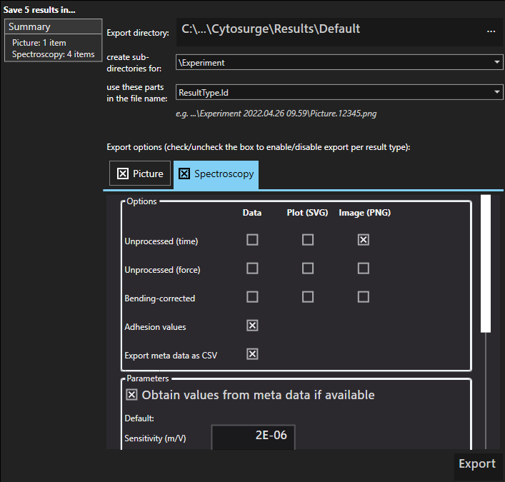
Here you can choose which details you would like to export and how to name the exported files.
Click on the export directory to change the directory where to export the result data. If this path is too long to display, it will be truncated - hover the mouse over the path to see the full one.
You can also control whether to create sub-directories. By default, the exported data will be placed in the sub-directory using the name of the current experiment. For result groups a subfolder for the grouped results will always be created.
Next, you can choose how to name the exported files. The default is to include the result type (e.g. picture, spectroscopy, …) and the unique database Id of the result in the name.
Finally the dialog allows you to select which result types you would like to export and offers a few export options depending on the result type.
Note
During export, the date of the exported file is set to the time at which the corresponding result was acquired. This may be useful to sort the exported files e.g. in Window’s File Explorer.
Exporting results associated with points
If exporting from the point-filter view, you can also choose to create sub-directories for each point group and point. Directories created for points will always include an Id of the point (this Id is different from the results’ Ids).
When exporting a point group an XML file containing details about the points will be created in the group’s sub-directory.
Export Formats
How data is written to the export destination is mainly controlled by built-in software parameters. However, following general rules apply:
- Spectroscopy data
-
Generally, axis positions are stored in [mm] - the encoder’s native format - time values in [s] and deflection values are in [V]. Values depend on the export configuration but overall the following units as used:
- Adhesion Interval [m]
- Adhesion Energy [J]
- Adhesion Force [N]
- Sensitivity [m/V]
- Approach Offset [V] - determined during bending correction
- Retract Offset [V] - determined during bending correction
- Data points: x is the absolute position value of the z-axis [mm]; y is the deflection value [V] corrected by the settings in the export configuration.
Deflection is within [-1,1]. The axis’ range depends on the exact stage model but usually has a range of around 60mm.
By default, the sensitivity and spring constant used to calculate the adhesion values are taken form the metadata stored alongside the result. This metadata may not be available if sensitivity and spring constant were not set when the data was recorded or when an older version of the software was used to record the data. In any case you have to specify default values for sensitivity and spring constant which will be used when no metadata is available or the meta data option is unchecked.
- Spectroscopy plot
-
An svg or png file that is sub-sampled according to the resolution specified in the export window
- Images
-
These image formats are available:
- Lossless (TIFF): exports a lossless tiff file of the image as captured from the camera (at the camera’s resolution and bit depth).
- Lossless (PNG): exports a png file of the image as captured from the camera (at the camera’s resolution and bit depth).
- Medium (JPEG) : creates a jpeg image with a high quality level, such that the information loss is low.
- High (JPEG): creates a jpeg image with a medium quality level to reduce the size of the exported file.
- Thermal tuning data
-
Collection of data blocks recorded at several kHz. Each line contains a time offset [s] and an ADC value within [0,220]
- Volume calculation report
-
A csv file listing the calculated volume per image
- Cantilever volume
-
A csv file listing the selected volume per point.
Exporting the related image highlighting the selection is optional.
- Metadata
-
Metadata associated with results as csv file
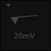
Dragging
Some tools are overlaid over the video feed. These can be moved by dragging the black handle bar on their right side.

Cancellation
Buttons that start an operation usually also terminate it on a subsequent click. This is indicated by a red cross which overlays the button when cancellation is possible.
An example with the approach button:
| State | Description |
|---|---|
 |
An operation is ready to be started |
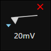 |
The operation is running - press again to abort |
 |
The operation is currently not available; either it is being stopped or another operation is running |
Arrow navigation
In various situations (e.g. during Laser Alignment) fine grained control over a movement is necessary. In this case an arrow navigation tool as depicted will be available.
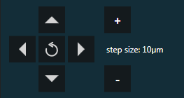
Clicking on the arrow keys will perform a movement in the corresponding direction by the distance indicated on the right by step size. The step size can be changed with the + and - buttons.
Clicking on the button will reset all axes to their initial position (this button may not be available in all situations).
Hint: Keyboard navigation
Instead of clicking the buttons the arrow keys (`←, →, ↑, ↓) on the keyboard can be used for navigation, the + and - keys on the keypad for step size control.
Number editor
Clicking on an editable number in the software brings up the number editor. You can change both the value and the unit of the current number. Changes become only effective once the number is applied.
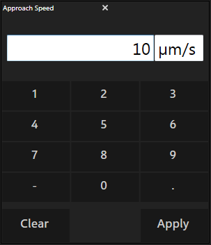
The number editor validates your input and gives feedback if, for example, your unit is not supported or your value is out of range.
Hint
You can use ‘u’ instead of ‘µ‘ (e.g. um = µm)
If the slider icon is present, you can click on it to show a slider instead of buttons to set your desired value.
Hint: Scientific notation
The number editor also supports scientific notation. E.g. one can write 1e-6 instead of 0.000001.
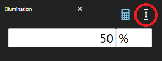
Quick Adjust
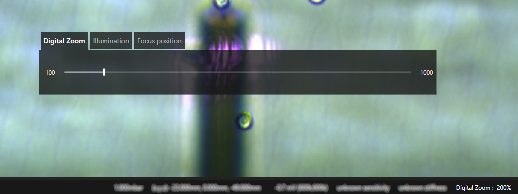
- Tool visible with activated parameter ‘Digital Zoom’ whose value is also listed in the statusbar.
This feature can be used to quickly adjust view-related parameters instead of changing them in the settings menu.
To open the tool, press Ctrl+Space. It remains open until Ctrl is released.
Pressing Space while keeping Ctrl pressed cycles through the individual parameters.
To change a parameter’s value, use either the slider or the mouse wheel.
After closing the tool the last active parameter can be adjusted without opening the tool by pressing Ctrl and using the mouse wheel.
For some parameters the range displayed in the tool is smaller than the full range of supported values. This allows for more fine-grained control of the value. In this case, the displayed range is re-adjusted and centered around the current value when the tool is re-opened. Moreover, you can continue changing the value when the slider reaches either the left or right limit by both continuing scrolling the mouse wheel or keeping the mouse button pressed when dragging the slider. In the latter case you can increase the speed with which the value is changed by moving the mouse further from the limit.
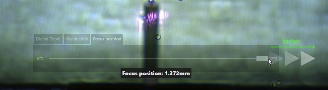
- Slider dragged to the far right continues changing the value while the arrows are shown.
Stage movement
Standard dragging
While looking at a sample, clicking and maintaining pressure on the mouse’s left button will trigger a dragging process. At that point, the cursor will change to a grabbing hand and any mouse movement will be followed by the stage.
To quickly move an object below the probe one can press the control key and double click on the target object.
Infinity movement
While the standard drag is the ideal way to carry out small movements, the need to travel longer distances within a well might arise. To this end, use the so called “infinity” drag. Click and maintain the mouse’s left button while hovering around the edge of the screen and you will trigger a constant movement in the opposite direction. Why the opposite direction? To enable you to switch between standard dragging and “infinity” movement seamlessly.
- A screenshot of an “infinity” movement indicated by the white arrow over a transparent border.
Boundaries
To prevent you from hitting a plate, a boundary checker is implemented for each plate type. As a result, you will see a red, transparent border appear whenever a boundary is reached while moving the stage, be it when dragging or in “infinity movement” mode.
- A screenshot of a boundary warning: the red arrows show the forbidden directions while the red, transparent border indicates a boundary was reached.
Point Overlay
Previously previously processed positions which have a result attached can be displayed as overlay on the video feed.
The overlay can be shown or hidden using the button at the bottom of the video feed.
Positions displayed in the overlay can be limited to positions processed
- since the software was started
- in the scope of the active exeperiment
- since a configurable time (click on the displayed time to change the range)
This also limits the positions displayed in the activity map of the navigation tool.
If positions are too close to be displayed on the video feed, a rectangle is displayed instead, indicating the number of positions within the represented area.
Data Plotting
The plotting module of the software gives you the possibility to visualize spectroscopy curves and spring constant measurements.
The plots
To begin with, there are several ways to look at a spectroscopy curve. These are accessible through the controls on the bottom-right of the module.
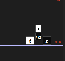
- Controls to modify the plotting logic of the displayed information. [t] for time, [z] for vertical distance.
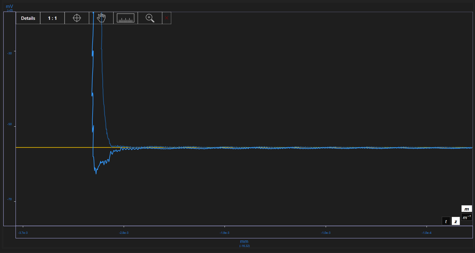
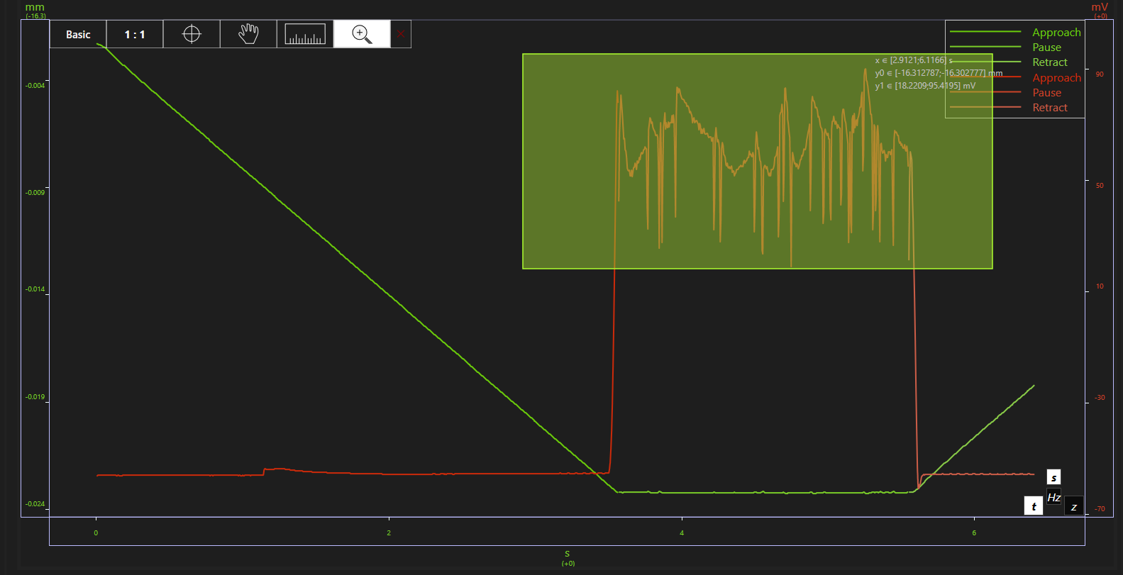
Time plot
The simplest display is a (t, z(t), V(t)) plot where z(t) stands for z axis position, while V(t) represents the position of the signal on the detection. The deflection value V(t) can be interpreted as follow: +/-1 Volt represents a cantilever fully bent away from/towards the sample.
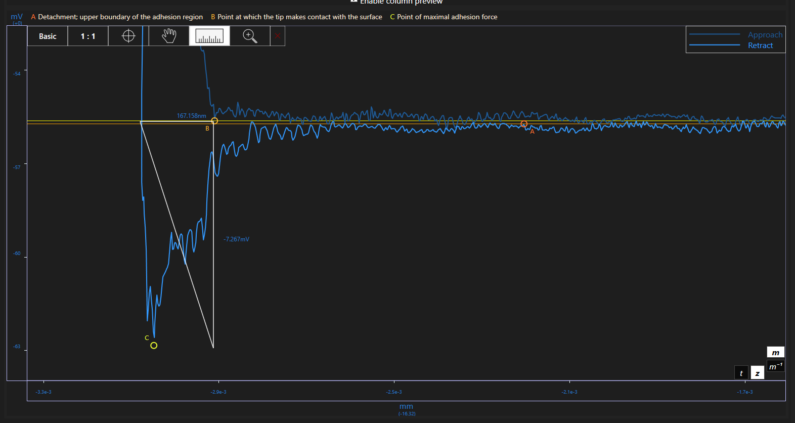
Force plot
The most readable display is a (z, V(z)) plot of the signal position on the detector against axis height. The closer the cantilever is to the surface, the more likely it is for the signal to change due to various interactions.
The y axis’ unit can be toggled by double-clicking the unit label on top of the axis. If sensitivity and stiffness are provided, this will cause values on the axis and in the plot to be multiplied according to the conversion factors.
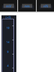
- Possible representation of units
The time plot is available either in absolute units or in their Fourier-transformed version. Selecting the [t] icon opens two sub-icons: [s] for seconds and [Hz] for Hertz. This enables you to take a peek at possible noise sources, for instance.

- Absolute units: noisy interval; Fourier spectrum: first noise frequency around 20Hz, second frequency peak at ca. 250Hz and following harmonics.
Data menu
A right-click over the plot will open a menu to choose the data you wish to display.
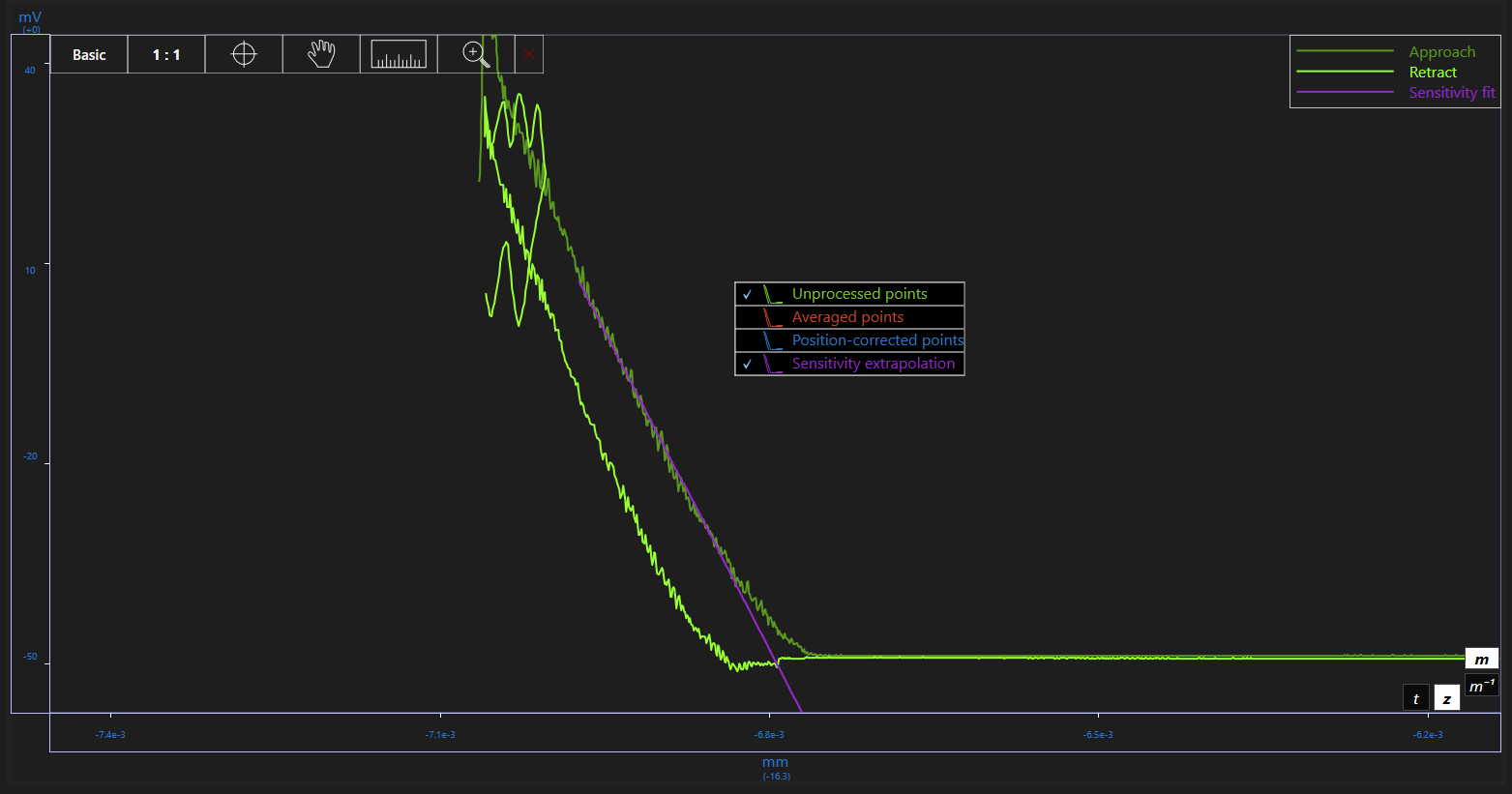
- Data menu: Choose to see processed/unprocessed data, fits or averages depending on what is available.
The toolbar
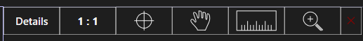
The toolbar displays some of the options at your dispositions:
- Basic/Details
- Unzoomed view
- Position reader
- Plot dragging
- Two-dimensional measurer/ruler
- Region zoom
Not included in the toolbar is the essential “scroll-zoom” that lets you zoom in and out at any moment using the mouse wheel.
Basic/detailed view
The basic/details button lets you toggle between a view with additional information such as curve legend, points, and a more sober view that displays only the curve.
- Basic view: the curves, the ranges, the controls and the toolbar.
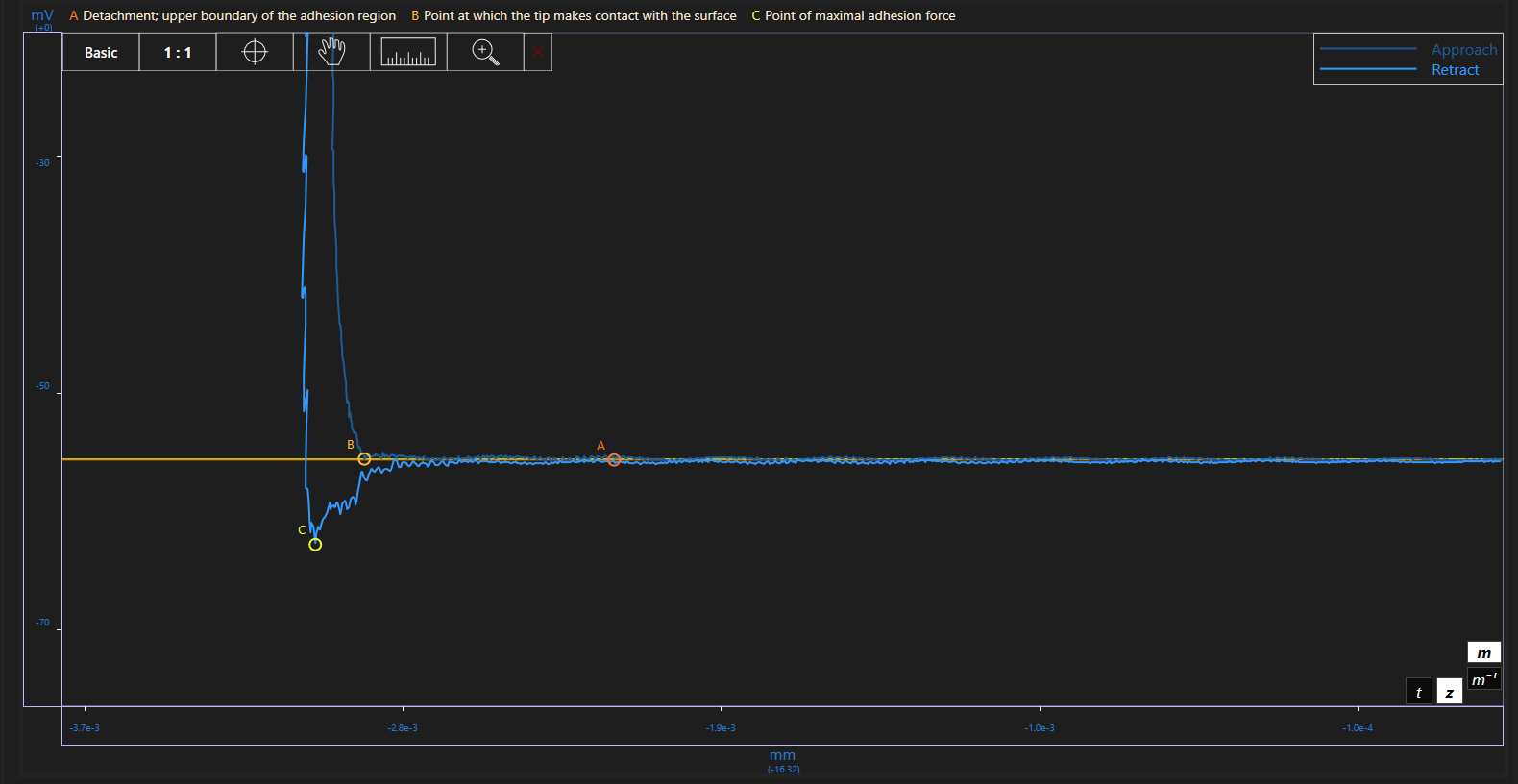
- Detailed view: special points, curve legend, point legend added to the basic view.
Unzoomed view
The button marked with 1:1 lets you go back to the unzoomed view directly in order to save you some scrolling.
Position reader
The target icon stands for a position reader that displays the position of your cursor translated in plot unit. To activate this feature, you can either click on the target icon or press on the space bar.

- Position reader: when the position reader is selected, a box appears next to your cursor to provide exact values on its position.
Drag
The grabbing hand stands for the dragging feature of the tool. You can either click on the hand icon and drag, or simply click, hold and move the mouse to drag the plot.

- Dragging: When dragging is selected, the cursor is a “grab-hand”; a click turns it into a “grabbing-hand”.
Measurer
Click on the ruler icon, then on a point on the plot to trigger the measuring tool. You can use it to get precise estimations of distances/intervals in the plot. This feature is also accessible by pressing “Ctrl” and clicking on a point in the plot.
- Measurer: Measuring an interval becomes easy using this option.
Region zoom
If you need to take a peak at a certain region of the plot, press on the magnifier icon, then select the region by clicking on a point and moving the mouse. This feature is also accessible by double-clicking and holding the left button of the mouse.
- Region zoom : Draw a rectangle to describe the region you want to further investigate.
Settings
| Settings Name | Description | Affected Components | Persistent |
|---|---|---|---|
Approach Setpoint |
The probe deflection value at which the approach will be stopped. Typically around 10 mV or 30 nN. Higher values are sometimes necessary if you have noise due to floating particles in the sample, as for example in cell medium. | Probe tool, Default value for workflows | No |
Approach Speed |
How fast the FluidFM probe approaches the sample. Higher values can drastically reduce the time to approach, but also increase the risk of probe damage. We recommend values around 5 µm/s. | No | |
Retract Speed |
The speed at which the probe is lifted away from the surface. | No | |
Safety Retraction |
The dafault distance by which the probe is automatically retracted after a successful approach. | Probe tool, Sensitivity measurements | No |
Long Distance Retraction |
The distance by which the probe is automatically retracted before the stage moves by at least 500µm with the probe close to the surface. | Injection, Cell Isolation and Spotting (including calibration) workflows | No |
Active Sensitivity |
[m/V] Check and/or adjust the sensitivity anytime. Beware that it is in [m/V], i.e. a value of 1.5 E-6 or 1.5 micron per Volt is not uncommon. You can type “E” to indicate the exponent of 10 when modifying the sensitivity. | No | |
Active Spring Constant |
[N/m] Check and/or adjust the active spring constant anytime. | No | |
Active Channel height |
The height of the microchannel inside the cantilever. | Extraction | No |
PI Parameters |
These parameters are used to keep the setpoint with a proportional-integral control loop once the probe is in contact with the surface. Too high parameters will cause the probe to oscillate, too low parameters will slow the system down. To optimize the PI parameters, monitor the cantilever deflection when in contact with the surface during a spectroscopy. | ||
Illumination |
The FluidFM Omnium has an integrated LED illumination. Set its value here. | Yes | |
Objective |
You can choose which objective you want to use here. When using a non-motorized microscope it is important to adjust this value yourself whenever changing the objective. The magnification is an important information for ARYA to know the right scale. | No | |
Optovar |
A magnifying optovar can enlarge details on some microscopes, it will however not increase the resolution. | No | |
Show Help Lines |
Choose whether to show help lines (a crosshair and a square indicating the size of a 100 by 100 µm area) in the center of the video view. | Yes | |
Idle Pressure |
The pressure that will be constantly applied by the pressure system in idle situations to prevent liquid from flowing through the cantilever in either direction. This value is automatically updated after probe filling. | Pressure tool, Default value for workflows | Yes |
Record Injection Data |
Whether to save spectroscopy curves of injection runs. | Injection workflow | Yes |
Auto Retract Lens |
Whether to automatically retract the lens when passing plate borders and restore the original focus distance on move completion. Users of non-motorized microscopes are adviced with a message to retract the lens. | Any move between plates | Yes |